By Pia Götz
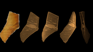
Figure 1: Rendered Micro-CT images of a shard of a Siegburg Stoneware depicted from different perspectives. © Pia Götz
What do a torn ligament in the ankle joint and an air bubble in a shard from the 16th century century have in common? Both can be determined and measured non-destructively. With a computer tomograph.
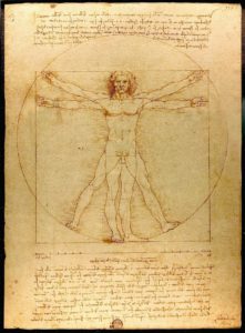
Figure 1: Anatomical drawing by Leonardo da Vinci. © WikiImages on Pixabay
We have all heard the term computer tomograph. Some of us may even have heard of it ourselves. With the help of computer tomography (CT for short), detailed images can be taken in medicine and the smallest changes in human tissue can be made visible. It is mainly used in the diagnosis of the skeletal system, the brain and internal organs and blood vessels. Doctors thus gain an insight into the inside of the body without having to open it. This is a clear advantage over old methods, which we would rather not imagine in retrospect, for example, in the early 16th century. Leonardo da Vinci’s detailed anatomical drawings, for example, are said to be based in part on dissections he performed himself. If only computer tomography had existed back then.
But wait – what exactly does all this have to do with a shard?
The technique, originally developed for medical use, is now also used in sciences outside medicine, for example at the MAPEX Center for Materials and Processes at the University of Bremen. Here, objects made of different materials are examined with an X-ray microscope. From tiny foraminifera (see Figure 2, left), to fibre and rock samples, to teeth (see Figure 2, right). And also a sherd from the 16th century. This article uses this shard to explain computed tomography in materials science.
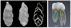
Figure 2: Example foraminifera from left: 3D view, virtual section and CT image slice. Tooth on the right with thickness measurement of the root canals. © MAPEX Wolf-Achim Kahl
History of computer tomography
Since the discovery of X-rays on 8 November 1895 by the German physicist Wilhelm Conrad Röntgen, human mankind is able to make use of electromagnetic waves in order to examine the body and other objects. For that purpose, the absorption behaviour of the different materials is used. This is based on the one hand on the density of the object to be examined and on the other hand on the composition of the chemical elements. “Heavier” elements with a high atomic number, i.e. a high number of protons in the atomic nucleus, are rather impermeable to X-rays, while “lighter” elements hardly absorb the radiation at all. The element calcium, for example, which is found in bones, has an atomic number of 20, which is significantly more protons than the element hydrogen, which has an atomic number of 1. The other elements in soft tissue, such as carbon, nitrogen and oxygen, also have a lower atomic number than calcium. Different densities of tissue thus absorb radiation to different degrees, creating a shadow image behind them. First on two-dimensional plates.
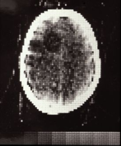
Figure 4: 1971: World’s first CT scan of a head at Atkinson Morley Hospital in London. In an 80×80 matrix. Each scan took 5 minutes per position. © Atkinson Morley Hospital
It was not until over half a century later, in 1971, that the first prototype of a CT scanner was presented. Although there had already been considerations to record objects from different angles, the lack of knowledge about the procedure for back-calculating the individual images made implementation impossible. In addition, the scientific community was not well networked at the time. Thus, the South African-US physicist Allan McLeod Cormack in Massachusetts and the British electrical engineer Sir Godfrey Newbold Hounsfield in England were working almost simultaneously on the same problem of back-calculating and reconstructing X-ray images.
Cormack was already working on the mathematical challenges of reconstruction in the 1950s. Even before this time, the Austrian mathematician Johann Radon had set a milestone for future generations in 1917. With his idea, the Radon transformation, he was able to show mathematically that a function can be reconstructed from infinitely many projections of the function. Only Cormack didn’t know about it. He later stated that he only found out about Radon’s work in 1972, so he had to find the solution himself.
The principle of the Radon transformation and the approximate solution for large systems of linear algebraic equations developed in 1937 by the Polish mathematician Stefan Kaczmarz are important building blocks of Cormack’s theoretical calculations. However, at the time he lacked the equipment and a computer to put his ideas into practice.
So in 1969, another person with the necessary financial means realised the first prototype of a CT scanner. Hounsfield was employed as an electrical engineer at EMI – yes, that’s right Electric and Musical Industries Ltd. For a long time one of the biggest record labels in the world. The rumour persists to this day that the Beatles, who were under contract to EMI at the time, made a considerable contribution to the development of computer tomography with the money they collected. In any case, EMI did not lack financial means. However, Hounsfield, for his part, had no knowledge of Cormack’s preliminary work and elaborately worked out the algorithms for image reconstruction himself.
Both scientists, one in the USA, the other in England, thus share two things in common besides their passion for computer tomography:
- Both could have saved themselves a great deal of time and work if publications could have been found in an online search at the time.
- Both share the Nobel Prize for Physiology and Medicine in 1979.
All’s well that ends well.
The making of a digital shard in the 21st century
The shard from the early 16th century, the time when da Vinci was still dissecting for his records, is placed on a rotatable plate, as shown in the schematic diagram in Figure 4. In contrast to what we know from hospitals, the X-ray source and detector do not rotate around the body part to be examined, but the shard rotates around its own axis, while the X-ray source and detector remain fixed in their positions.
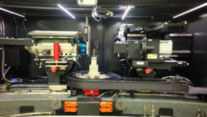
Figure 5: X-ray microscope at MAPEX, from left: X-ray source, rotatable sample holder, various detectors. © Pia Götz
The X-ray source, on the left of the shard, generates X-rays. The detector, to the right of the shard, measures the intensities of the radiation after it has passed through the object and converts it first into visible light and then into electrons with a photodiode. The distances between the individual measuring points on the detector determine the pixel size and the spatial resolution. All the pixels of an image are combined to form a 2D overall image, also called a projection. The intensities for each pixel are represented as grey values, resulting in a black and white image. The more opaque a spot in the object, the higher the attenuation of the output radiation, the lower the radiation that the detector perceives at the spot.
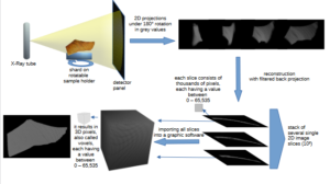
Figure 6: How a digital object is made from an analogue shard: The X-ray source generates X-rays that pass through the shard. The projection is recorded by the detector. The plate rotates, the shard is X-rayed from a different angle and measured again. By means of an algorithm, all projections are converted into a stack of images. This image stack, consisting of many layers, is loaded into a software for further processing and analysis. © Pia Götz
After each individual measurement, the plate with the shard rotates a tenth of a degree further until the object has been completely measured once. This produces around 2,000 X-ray images from different angles. As a rule, 180° is sufficient as a rotation, since everything above 180° has already been measured, only from the other side.
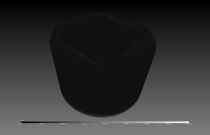
Figure 7: Image stack as a 3D object. Air with low grey values is initially displayed in black, edge of plastic container visible. © Pia Götz
The projections from the different angles are then calculated back to a 3D object using an algorithm. The result is called a reconstruction. In addition to the measured intensities, this also requires the geometry of the measurement set-up, i.e. how far apart the X-ray source, object and detector were from each other. After the so-called back projection, our example sherd from the 16th century is now available as a stack of grey-scale images of individual slices. Virtual slices through the object. This also explains the term tomography. Thus τομή, tome in ancient Greek means ‘cut’ and γράφειν, graphein ‘to write’.
A clay shard big time
Measuring a sherd can take several hours, depending on its size and the desired resolution. The reconstruction also takes a lot of time and also requires enormous computing power. The individual projections of a small shard can take up to 20 GB of space. By comparison, the film Matrix, with its 2 hours 16 minutes in the 4K Ultra HD version, takes up less space on the hard drive.
65,536 shades of grey
If the once analogue object is now on the hard disk in digital slice form, it can be loaded into a graphics programme. But what happens then? The image pixels now become volumetric pixels, also called “voxels”, and are initially represented as a solid, grey block. This is because everything that we define as non-shear but falls within the measurement volume is also generally measured. This includes the air, the container in which the shard is located and the cushioning material that protects the shard from slipping during the entire measuring process. So for the time being, the computer knows no difference between the different materials. Black and white with all the 65,534 nuances in between are displayed.
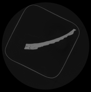
Figure 8: Grey scale of the shard in the plastic container with paper for padding, pixel values are between 0 (black) and 65,535 (white). © Pia Götz
Only by fading out a certain range of grey values do properties become visible that were previously hidden. If we now virtually fade out the air, we see the shard in its paper nest in a plastic container, just as it was embedded in the device during the measuring process. For further processing, it is advantageous to reduce the image volume. Therefore, segmentation is carried out: the grey values of interest, i.e. those of the shard, are marked. The surrounding rest is removed. Thus, the image volume shrinks considerably.
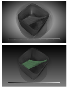
Figure 9: 3D image of the shard in the plastic container with semi-transparent air and padding. Below: Segmentation of the grey value range of the shard. © Pia Götz
From grey to colourful
If we now want to look further into the interior of the shard, i.e. look at its inner (grey) values, carefully selected value ranges can not only be faded in or out, but also marked in colour. In addition, contrast settings can be helpful in the visualisation. We are now entering the virtual realm of rendering. To render something means to reproduce or present something. It is the interplay of light and shadow in an animated film scene. It is also used in the visualisation of computer games. The result is a virtual spatial model that artistically creates the viewer’s line of vision, lighting effects and depth-of-field effects based on raw data.
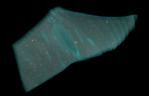
Figure 10: Semi-transparent visualisation of the shard. Air pockets become visible through rendering. Particles with higher X-ray absorption are marked in yellow. © Pia Götz
Consequently, colour and material properties, such as reflections on the surface, can be changed at will, completely detached from the analogue object. In this way, air inclusions in the shard are also made digitally visible when the transparency of the surrounding material is increased. The shape and distribution of these air inclusions allow conclusions to be drawn about the manufacturing methods at the time. The composition of the material can also be assessed in a similar way. Let’s just look at the yellow particles in the illustration. These are areas that have a higher grey value. So the material here is more opaque to X-rays than the surrounding material. What could be the cause of this? What other abnormalities can we detect? What material science insights do we draw from this and what use is the rendering for other scientific disciplines? Another Science Blog article will follow soon, which will go on a journey through time to answer precisely these and other exciting questions.
Sources
History of computed tomography:
Seynaeve PC, Broos JI. [The history of tomography]. J Belge Radiol. 1995 Oct;78(5) 284-288. PMID: 8550391.
https://en.wikipedia.org/wiki/History_of_computed_tomography
Image sources
First CT scan of a head – http://www.impactscan.org/CThistory.htm
Example images of foraminifera and tooth: Wolf-Achim Kahl, MAPEX Bremen, wakahl@uni-bremen.de
All other visualisations: Pia Götz, MAPEX Bremen, piagoetz@uni-bremen.de
Visualisation software: Dragonfly ORS 2021.3 – https://www.theobjects.com/index.html


Leave a Reply